First published in Analytics Vidhya
Co-authored by Ioannis Tsamardinos (JADBio), Iordanis Xanthopoulos (Univ. of Crete, Greece), Vassilis Christophides (ENSEA, France)

---

What is AutoML?

Automated Machine Learning, or AutoML, promises to automate the machine learning process end-to-end. It is a fast-rising, ultra-hot sub-field of machine learning and data science. AutoML platforms try hundreds or even thousands of different ML pipelines, called configurations, combining algorithms for the different analysis steps (transformations, imputation, feature selection, and modeling) and their corresponding hyper-parameters. They often deliver models that beat the experts and win competitions, all with a few mouse clicks or lines of code.

The Need to Estimate Performance

However, obtaining a model is never enough! One cannot trust the model for predictions unless there are guarantees of predictive performance. Is the model almost always accurate or closer to random guessing? Can we depend on it for life and death decisions in the clinic or business decisions that cost money? Having reliable estimates of out-of-sample (on new, unseen samples) performance is paramount. A good analyst would provide them for you, and so should an AutoML tool. Do existing AutoML libraries and platforms return reliable estimates of the performance of their models?

What’s the size of the test set?

Well, some AutoML tools do not return any estimates at all! Take, for example, what is arguable, the most popular AutoML library: auto sklearn. Its authors suggest that to estimate performance, you hold out a separate, untainted, and unseen by the library test set strictly to estimate the final model’s performance. What tools like auto sklearn essentially offer is a Combined Algorithm Selection and Hyper-parameter optimization (CASH) or Hyper-Parameter Optimization (HPO) engine. They may be extremely useful and population but only partially implement the AutoML vision. After all, if you are required to decide on the optimal test size, write the code to apply the model, and the code to do the estimation, then the tool is not fully automatic. Deciding on the optimal test size is not trivial. It requires machine learning skills and knowledge. It requires an expert. Should you leave out 10%, 20%, or 30% of the data? Should you partition randomly or stratify the partition according to the outcome class. What if you have 1,000,000 samples? What percentage would you leave out? What if you have 1,000,000 samples and the positive class has a prevalence of 1 out of 100 000? What if you have a censored outcome like in survival analysis? How much is enough for your test set so that estimation is accurate? How do you calculate the confidence intervals of your estimate? Once you let the user decide on the test set estimation, you cannot claim anymore that your tool “democratizes” machine learning to non-expert analysts.

Losing Samples to Estimation

Having a separate hold-out test, however, creates an additional, deeper, more serious problem. The held-out data are “lost to estimation.” It could be precious data that we had to pay handsomely to collect or measure, data that we had to wait a significant time to obtain, and we just use them to gauge the effectiveness of a model. They are not employed to improve the model and our predictions. In many applications, we may not have the luxury to leave out a sizable test set! We need to analyze SARS-CoV-2 (COVID-19) data as soon as we observe the first few deaths. Not after we wait long enough to have 1000 victims to “spare” just for performance estimation. When a new competitor product is out, we need to analyze our most recent data and react immediately, not wait until we have enough clients dropping out. “Small” sample data are important too. They are out there, and they will always be out there. Big Data may be computationally challenging, but small sample data are statistically challenging. AutoML platforms and libraries that require an additional test set are out of the picture for the analysis of small sample size data.

From Estimating Performance of Models to Estimating Performance of Configurations

Other AutoML tools do return performance estimates based on your input data only. They do not require you to select test set sizes, truly automating the procedure and paying justice to their name. Here is the idea: the final model is trained on all the input data. On average, since classifiers improve with sample size, this will be the best model. But then, we do not have any samples for estimation. Well, cross-validation and similar protocols (e.g., repeated hold-out) use proxy models to estimate the performance of the final model. They train many other models produced with the same configuration. So, they do not directly estimate the performance of the prediction model; they estimate the performance of the configuration (learning method, pipeline) that produces the model. But, can you trust their estimates? Which brings us to the so-called “winner’s curse.”

Estimating Performance of a Single Configuration

We will illustrate an interesting statistical phenomenon with a small, simulated experiment. First, we will try to estimate the performance of a single configuration, consisting of a classifier with specific hyper-parameters, say 1-Nearest Neighbor. I simulate a test set of 50 samples for a binary outcome with 50–50% distribution. I assume my classifier has an 85% chance of providing the correct prediction, i.e., an accuracy of 85%. The next figure, panel (a), shows the accuracy estimate I obtained during my first try. I then generate a second (b) and a third (c) test set and corresponding estimates.

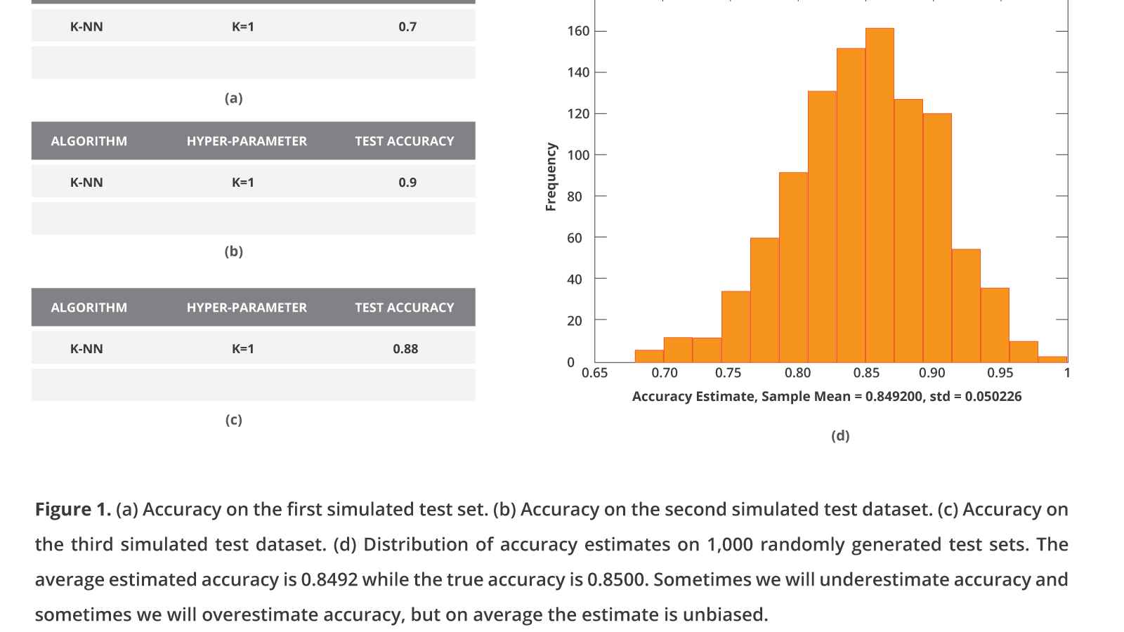
Sometimes my model is a bit lucky on the specific test set, and I estimate a performance higher than 0.85. In fact, there is one simulation when the model got right in almost all 50 samples and derived a 95%-100% accuracy. Other times, the model will be unlucky on the specific test set, and I will underestimate the performance, but on average, the estimate will be correct and unbiased. I will not be fooling myself, my clients, or my fellow scientists.

The Winners’ Curse (or Why You Systematically Overestimate)

Now, let us simulate what AutoML libraries and platforms actually do, which is try thousands of configurations. For simplicity, I presume I have just 8 configurations (instead of thousands) of 3 different algorithms (K-NN, Decision Tree, and Simple Bayes) matched with some hyper-parameter values. Each time I apply all of them, estimate their performance on the same test set, select the best one as my final model, and report the estimated performance of the winning configuration. In the simulation, I assume all configurations lead to equally predictive models with 85% accuracy.

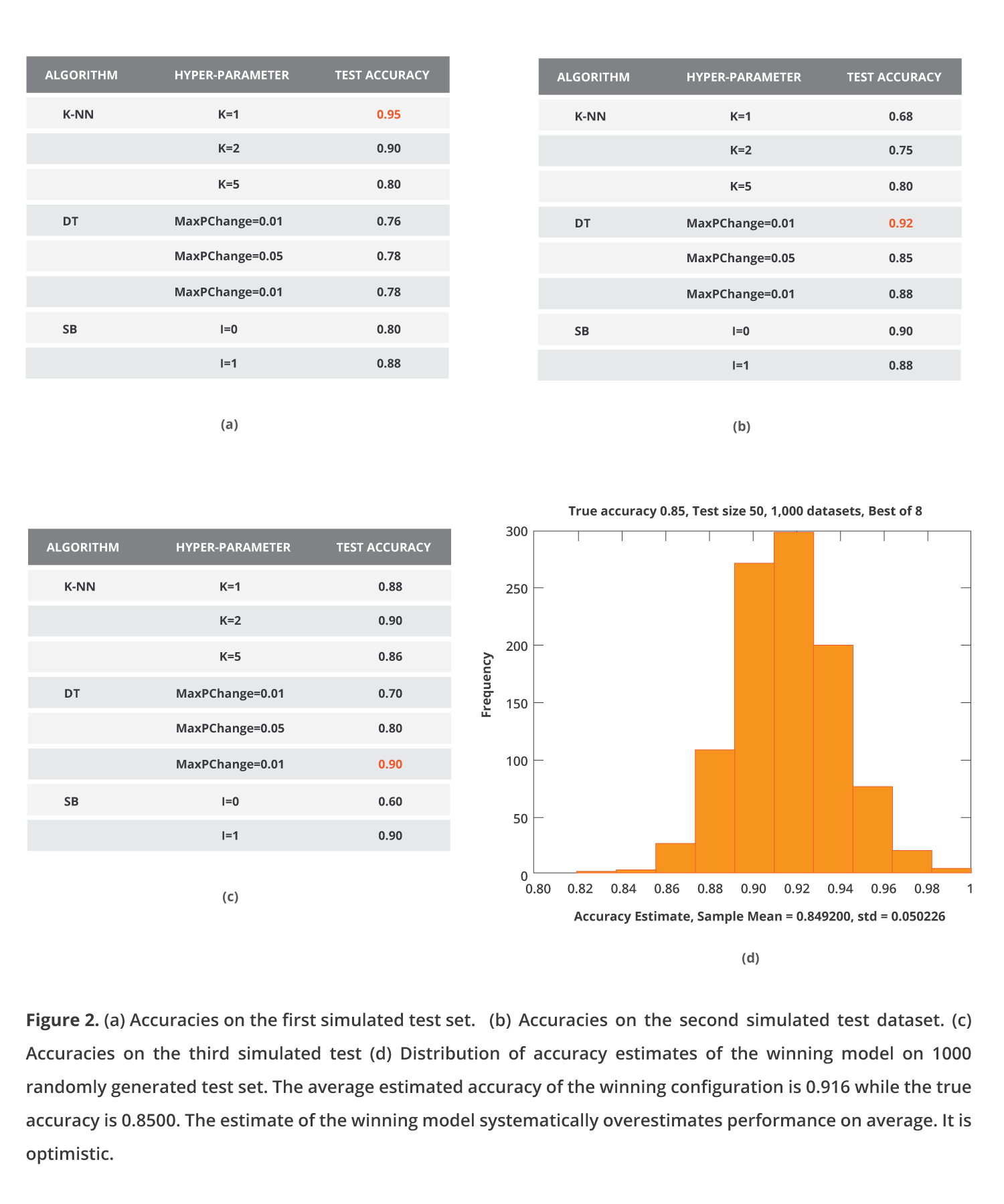
What happens after the 1000 simulations? On average, my estimate is 0.916, while the true accuracy is 0.85. I systematically overestimate. Do not kid yourself; you will get the same results with cross-validation. Why does this happen? The phenomenon is related to the “winner’s curse” in statistics, where an effect size optimized among many models tends to be overestimated. In machine learning, the phenomenon was first discovered by David Jensen and named “the multiple induction problem” [Jensen, Cohen 2000]. But, let’s face it “winner’s curse” is cooler (sorry David). Conceptually the phenomenon is similar to multiple hypothesis testing. We need to “adjust” the produced p-values using a Bonferroni of False Discovery Rate procedure. Similarly, when we cross-validate numerous configurations, we need to “adjust” the cross-validated performance of the winning configuration for multiple tries. So … when you cross-validate a single configuration, you obtain an accurate estimate of performance (actually, it is a conservative estimate of the model trained on all data); when you cross-validate multiple configurations and report the estimate of the winning one, you overestimate performance.

Does it Really Matter?

Is this overestimation really significant, or just of academic curiosity? Well, when you have a large and balanced dataset, it is unnoticeable. On small sample datasets or very imbalanced datasets where you have just a few samples for one of the classes, it can become quite significant. It can easily reach 15–20 AUC points [Tsamardinos et al. 2020], which means your true AUC being equal to random-guessing (0.50) and you report 0.70, considered respectable and publishable performance for some domains. The overestimation is higher (a) the smaller the sample size for some of the classes, (b) the more configurations you try, (c) the more independent the models produced by your configurations, and (d) the closer to random guessing is your winning model.

Can Overestimation Be Fixed? Can We Beat Winner’s Curse?

So, how do we fix it? There are at least three methodologies. The first one is — you guessed it — to hold out a separate test set, let us call it Estimation Set. The test sets during cross-validation of each configuration are employed for selecting the best one (namely for tuning) and are “seen” by each configuration multiple times. The Estimation Set will be employed only once, just to estimate the performance of the final model, so there is no “winner’s curse.” But, then, of course, we fall back into the same problem as before “losing samples to estimation.” The second method is to do a nested cross-validation [Tsamardinos et al., 2018]. The idea is the following: we consider the selection of the winning model as part of our learning procedure. We now have a single procedure (meta-configuration if you’d like) that tries numerous configurations, selects the best one using cross-validation and trains the final model on all input data using the winning configuration. We now cross-validate our single learning procedure (which internally also performs cross-validation on each configuration; hence, the term nested). Nested cross-validation is accurate (see Figure 2 in [Tsamardinos et al. 2018]) but quite computationally expensive. It trains O(C⋅K2) models, where C is the number of configurations we try and K the number of folds in our cross-validations. But fortunately, there is a better way; the Bootstrap Bias Corrected CV or BBC-CV method [Tsamardinos et al. 2018]. BBC-CV is as accurate in estimation as nested cross-validation (Figure 2 in [Tsamardinos et al. 2018]) and one order of magnitude faster, namely trains O(C⋅K) models. BBC-CV essentially removes the need for having a separate Estimation Set.

So, Can We Trust AutoML?

Back to our motivating question: can we trust AutoML? Despite all the work on AutoML, dozens of papers, competitions, challenges, and comparative evaluations, nobody has checked so far whether these tools return accurate estimates? Nobody, that is, until a couple of our recent works [Xanthopoulos 2020, Tsamardinos et al. 2020]. In the following figure, we compare two AutoML tools, namely TPOT [Olson et al. 2016] and our own Just Add Data Bio, or JADBio [Tsamardinos et al. 2020] (www.jadbio.com) for short. TPOT is a commonly used, freeware AutoML library, and JADBio is our commercial AutoML platform employing BBC-CV. JADBio was designed with these estimation considerations in mind and specifically to encompass small-sample, high-dimensional biological data. Given that models learned from biological data may be employed in critical clinical applications, e.g., to predict therapy response and optimize treatment, we were really striving to return accurate performance estimates.

We tried both systems on 100 binary classification problems from openml.org, spanning a wide range of sample size, feature size, and balance ratios (details in [Xanthopoulos 2020]). Each dataset was split in half, one to feed the AutoML tool and obtain a model and a self-assessed estimate (estimate of the model assessed by the AutoML platform, called Train Estimate), and one on which to apply the model (estimate of the model on the test set, called Test Estimate). The metric of performance was the AUC. Each point is an experiment on one dataset. Red dots are points below the diagonal, where the Test Estimate is lower than the training estimate, i.e., overestimated performances. The black dots are points above the diagonal, where performance is underestimated.

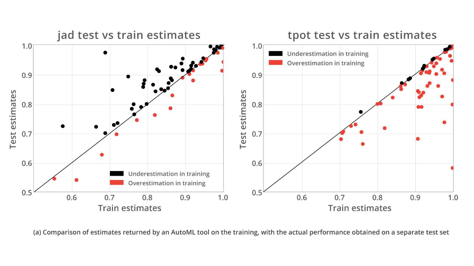TPOT seriously overestimates performance. There are datasets where the tool estimates model’s performance to be 1.0! In one of these cases (lowest redpoint), the actual performance on the test is less than 0.6, dangerously close to random guessing (0.5 AUC). It is obvious that you should be skeptical of TPOT’s self-assessed estimate. You need to lose samples to a hold-out test set. JADBio on the other hand systematically underestimates performance somewhat. The highest black point in the middle of its graph gets close to 1.00 AUC on the test but estimated performance at less than 0.70 AUC. On average JADBio’s estimates are closer to the diagonal. The datasets in this experiment have more than 100 samples and some over tens of thousands. In other, more challenging experiments, we tried our system JADBio on 370+ omics datasets with sample sizes as small as 40 and the average number of features at 80,000+. JADBio, using the BBC-CV, does not overestimate performance [Tsamardinos et al. 2020]. Unfortunately, it is not only TPOT that exhibits this behavior. Additional similar evaluations and preliminary results indicate that it could be a common problem with AutoML tools [Xanthopoulos 2020].

Don’t trust AND verify

In conclusion, first, beware of the self-assessment of performance of AutoML tools. It is so easy to overestimate performance when you automate analysis and generate thousands of models. Try your favorite tool on some datasets where you completely withhold part of the data. You need to do it multiple times to gauge the average behavior. Try challenging tasks like small-sample or highly-imbalanced data. The amount of overestimation may depend on meta-features (dataset characteristics) like the percentage of missing values, percentage of discrete features, number of values of the discrete features, and others. So, try datasets with similar characteristics like the ones you typically analyze! Second, even if you do not use AutoML and you code the analysis yourself, you may still produce numerous models and report the unadjusted, uncorrected cross-validated estimate of the winning one. The “winner’s curse” is ever-present to haunt you. You would not want to report a highly inflated, over-optimistic performance to your client, boss, professor, or paper reviewers, would you? … Or, would you?

References
[Jensen D.D. and Cohen P.R. (2000) Multiple Comparisons in Induction Algorithms. Mach. Learn., 38, 309–338. ]
[Tsamardinos I., Charonyktakis P., Lakiotaki K., Borboudakis G., Zenklusen J.C., Juhl H., Chatzaki E. and Lagani V. (2020) Just Add Data: Automated Predictive Modeling and BioSignature Discovery. bioRxiv, 10.1101/2020.05.04.075747]
[Tsamardinos I., Greasidou E. and Borboudakis G. (2018) Bootstrapping the out-of-sample predictions for efficient and accurate cross-validation. Mach. Learn., 107, 1895–1922.]
[Iordanis Xanthopoulos, M.Sc. Thesis, Computer Science Department, University of Crete, 2020]
[Olson R.S., Bartley N., Urbanowicz R.J., and Moore J.H. (2016) Evaluation of a tree-based pipeline optimization tool for automating data science. In GECCO 2016 — Proceedings of the 2016 Genetic and Evolutionary Computation Conference. ACM Press, New York, New York, USA, pp. 485–492.]

---