This website uses cookies to improve your experience. We'll assume you're ok with this, but you can opt-out if you wish. Read More
Ioannis Tsamardinos, Paulos Charonyktakis, Georgios Papoutsoglou, Giorgos Borboudakis, Kleanthi Lakiotaki, Jean Claude Zenklusen, Hartmut Juhl, Ekaterini Chatzaki & Vincenzo Lagani
npj Precision Oncology volume 6, Article number: 38 (2022)
doi: https://doi.org/10.1038/s41698-022-00274-8
JADBio’s AutoML approach can accelerate precision medicine and translational research. Specifically, it could facilitate the discovery of novel biosignatures and biomarkers leading to new biological insights, precision medicine predictive models, drug targets, and non-invasive diagnostics in cancer or other conditions.
FEATURE SELECTION FOR KNOWLEDGE DISCOVERY
In supervised learning, methods falling in the class of feature selection (a.k.a., variable selection or attribute selection), can be coupled with predictive modeling algorithms to identify (bio) signatures, defined as minimal-size subsets of molecular and other biological measurements that collectively lead to optimal predictions. Identifying such predictive signatures is of major importance for knowledge discovery, gaining intuition into molecular pathophysiological mechanisms, identifying novel drug targets, or designing diagnostic/prognostic assays with minimal measuring requirements.
Feature selection for knowledge discovery is often the primary goal in an analysis and the predictive model is just a side-benefit. Feature selection is different from differential expression analysis: feature selection examines feature correlations in combination (multivariately) and not individually. Not only it removes irrelevant features, but also features that are redundant for prediction given the selected ones.
The Problem with existing AutoML tools AutoML tools try to automate the analysis and predictive modeling process end-to-end in ways that provide unique opportunities for improving healthcare. They automatically try thousands of combinations of algorithms and their hyper-parameter values to obtain the best- possible model. However, state-of-the-art AutoML tools do not cover all the analyses needs of the translational researcher. Firstly, they do not focus on feature selection. As a rule, they return models that employ and require to measure all molecular quantities in the training data to provide predictions, thus hindering interpretation, knowledge discovery, and the ability to translate to cost-effective benchtop assays. Secondly, they do not focus on providing reliable estimates of the out-of-sample predictive performance (hereafter, performance) of the models. The latter is particularly important to a practitioner gauging the clinical utility of the model. Thirdly, they do not provide all information necessary to interpret, explain, make decisions, and apply the model in the clinic.
Focusing on reliable performance estimation, we note that it is particularly challenging in omics analyses for at least three reasons:
- The low-sample size of typical omics datasets. It is not uncommon for biological datasets to contain fewer than 100 samples: as of October 2021, 74.6% of the 4348 curated datasets provided by Gene Expression Omnibus count 20 or fewer samples. This is typical in rare cancers and diseases, in experimental therapy treatments, and whenever the measurement costs are high. When sample size is low, one cannot afford to hold out a significant portion of the molecular profiles for statistical validation of the model.
- Trying multiple machine learning algorithms or pipelines to produce various models and selecting the best-performing one, leads to systematically overestimating its predictive performance (bias). This phenomenon is called the “winner’s curse” in statistics, and the multiple comparisons in induction algorithms problem, in machine learning.
- Omics datasets measure up to hundreds of thousands of features (dimensions). Such high dimensional data are produced by modern biotechnologies for genomic, transcriptomic, metabolomic, proteomic, copy number variation, single nucleotide polymorphism (SNP) GWAS profiling, and multi-omics datasets that comprise multiple modalities. The combination of a high number of features (p) and a low-sample size (n), or as it is called “large p, small n” setting, is notoriously challenging as it has been repeatedly noted in statistics and bioinformatics leading to problems of model overfitting and performance overestimation. Such challenges have been recently noted in the precision medicine research community as well.
You can read the full research paper on Nature Precision Oncology or read a summary version below.
Scope
JADBio is qualitatively compared against auto-sklearn, TPOT, GAMA, AutoPrognosis, and Random Forests, demonstrating that it provides a wealth of unique functionalities necessary to a translational researcher for decision support and clinically applying a model. A case-study on the microbiome of colorectal cancer is presented to illustrate and demonstrate JADBio’s functionalities. JADBio is also comparatively and quantitatively evaluated on 360 public biological datasets, spanning 122 diseases and corresponding controls, from psoriasis to cancer, measuring metabolomics, transcriptomics (microarray and RNA-seq), and methylomics. It is shown that, on typical omics datasets, JADBio identifies signatures with just a handful of molecular quantities, while maintaining competitive predictive performance. At the same time, it reliably estimates the performance of the models from the training data alone, without losing samples to validation. In contrast, several common AutoML packages are shown to severely overestimate the performance of their models.
Data
5 cohorts containing 575 samples (285 colorectal cancer cases, 290 healthy controls). Wirbel, J. et al. Meta-analysis of fecal metagenomes reveals global microbial signatures that are specific for colorectal cancer. Nat. Med. 25, 679–689 (2019). https://www.nature.com/articles/s41591-019-0406-6
Tasks/Analyses
The analysis tasks were:
a. to create a predictive, diagnostic model for colorectal cancer given a microbial gut profile,
b. to estimate the predictive performance of the model,
c. to identify the biosignature(s) of microbial species that predict colorectal cancer, and
d. to apply the colorectal cancer model on new data. Particularly, we use each cohort to build a predictive model and every other cohort as its external validation set.
RESULTS
a. Analyzing colorectal cancer microbiome data
The detailed set of results is presented in Supplementary Table 1. Overall, JADBio analyses deliver similar performances as in the original publication, with the maximum difference between original and JADBio analyses being 0.08 AUC points. However, note that JADBio requires minimal human effort and selected fewer predictive features on average (up to 25). The number of features used in Wirbel et al. for each model cannot be extracted as they use an ensemble of models’ approach; for all practical purposes their models employ the full set of 849 features. Using all measured biomarkers in the model limits the knowledge discovery aspect of their analysis and their application to designing diagnostic assays.
A diagnostic model instance for colorectal cancer given a microbial gut profile
The configuration that produces the best-performing model on the CN cohort is reported in Fig. 1a. It produces a non-linear model, specifically, a Random Forest that includes 1000 different decision trees. If “Interpretability” is selected as criterion for this analysis, the best interpretable model is a linear Ridge Regression type of model (Fig. 1b), whose standardized coefficients are shown in Fig. 1c.
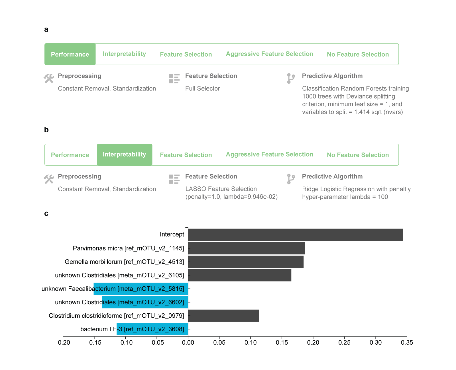
Fig. 1 The best performing and best interpretable model trained on the China (CN) cohort.
a Winning configuration that leads to the production of the final best-performing model when applied to all training data. It is produced by first applying removal of constant-value features and standardization of all features, followed by including all features in the model (FullSelector, i.e., no feature selection), and then modeling using the Random Forest algorithm. The hyper-parameter values to use are also shown. b Configuration that leads to the production of the best interpretable model. It is a linear Ridge Logistic Regression type of model, preceded by a Lasso regression for feature selection. c The interpretable model can be visualized, in contrast to the best-performing one. JADBio shows the standardized coefficients of the model for each selected feature and the intercept term.
b. Estimating the predictive performance of the colorectal cancer model
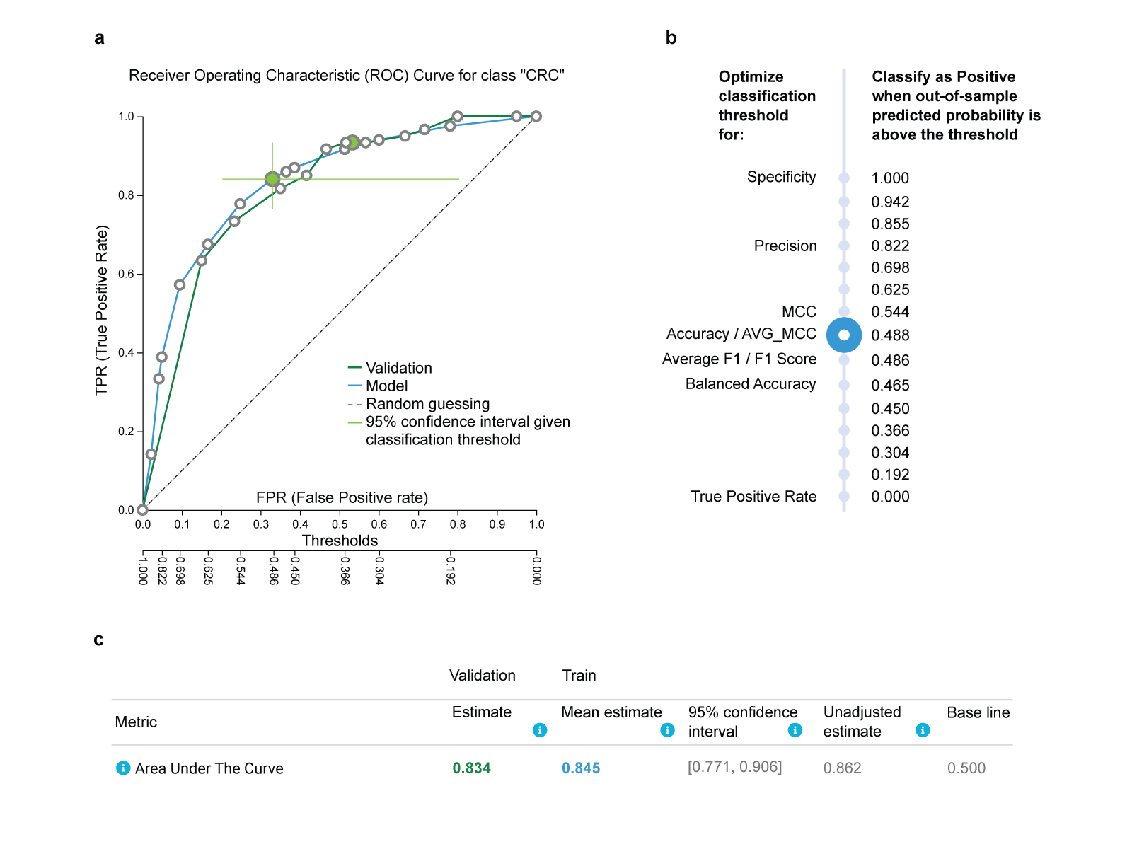
Fig.2 Predictive performance of the winning model optimized for Feature selection, trained on the China (CN) cohort and validated on the Germany (DE) cohort.
a. The Receiver Operating Characteristic (ROC) curve estimated on the training set and controlled for trying multiple different configurations is shown as the blue line. It shows all trade-offs between False Positive Rate (top x-axis) and True Positive Rate (y-axis) for all different classification thresholds (bottom x-axis). By clicking on a circle, a corresponding threshold is selected. The user can see how metrics of performance are affected, which facilitates selection of the clinically optimal threshold. The green cross shows the confidence intervals in each dimension for that point on the ROC. The ROC curve achieved by the model’s predictions on the DE cohort used as an external validation set is shown as the green line. It closely follows the blue line estimated from the training. b. A list of different thresholds suggested by JADBio and the corresponding metric of performance that they optimize. E.g., accuracy is optimized for threshold 0.488, while balanced accuracy is optimized for 0.465. c. The threshold-independent metric ROC Area Under the Curve (AUC) as estimated by the training (bold blue) and achieved on the validation (bold green) is reported along with its confidence intervals. Its unadjusted estimate (i.e., not adjusted for trying multiple configurations) is also reported and is expected to be optimistic on average. All other estimates computed by JADBio, including but not limited to accuracy, precision, recall (not shown in the figure) are adjusted for trying multiple configurations as well.
c. Identifying the biosignature(s) of microbial species that predict colorectal cancer
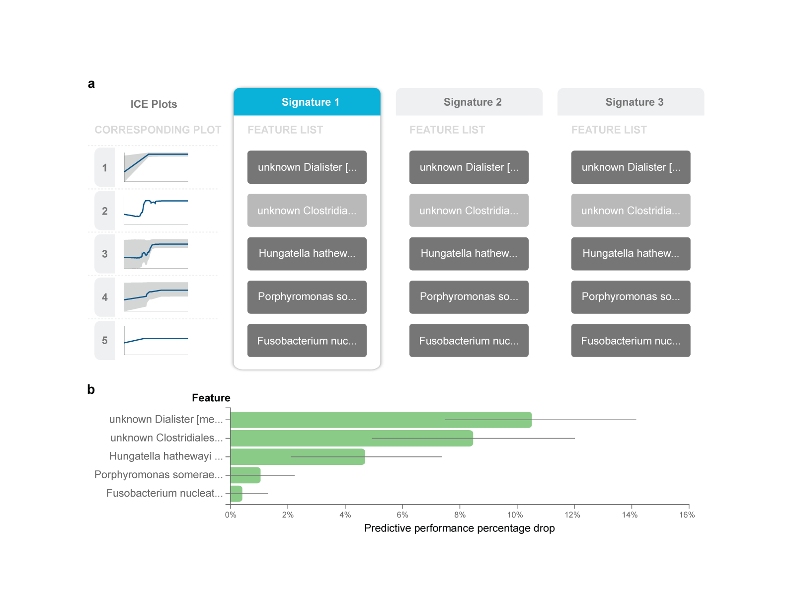
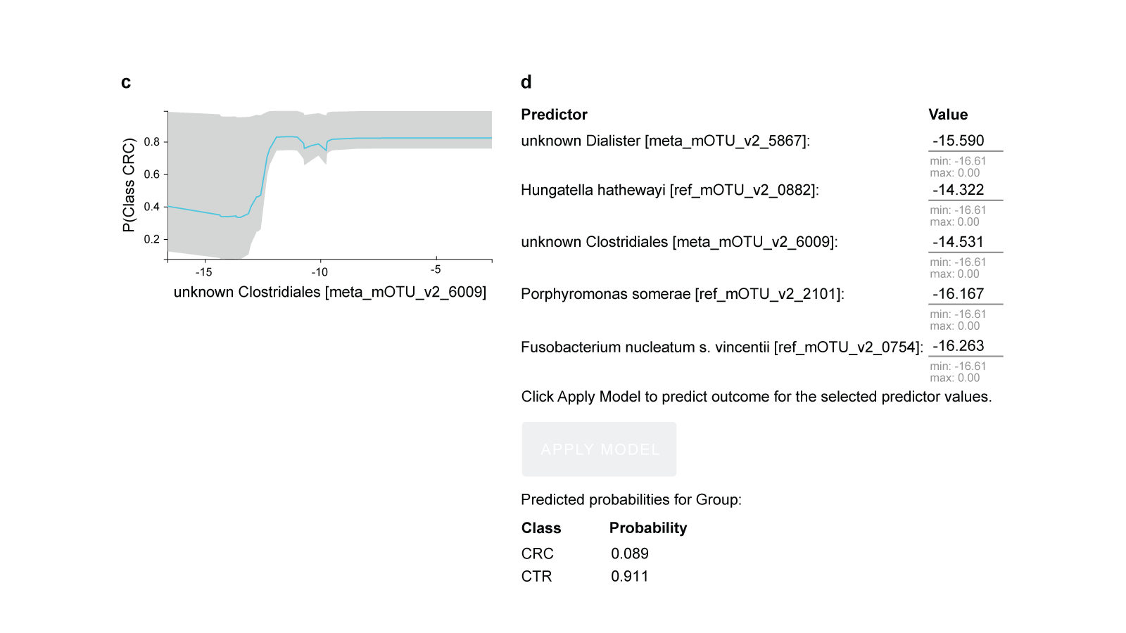
Fig.3 Feature selection (biosignature discovery) results for the best-performing model using the France (FR) cohort as training data.
a. There are three biosignatures identified, each containing five features. Each signature leads to an optimally predictive model. They share four features, while the second feature varies across signatures. b. Feature importance plot, assessing the relative drop in performance if each feature is dropped from the signature and the rest are retained. c. The Individual Conditional Expectation (ICE) plot for the ‘unknown Clostridiales [meta_mOTU_v2_6009]’: the higher its abundance, the higher the probability of colorectal cancer. Note that the trend is non- linear and non-monotonic (close to step function). d. The manual application of the model to get predictions for a fictional new sample is shown. Values are log-transformed relative concentrations, which can be negative if the original numbers are smaller than the logarithm base.
JADBio performs feature selection (biosignature discovery) simultaneously with modeling to facilitate knowledge discovery. JADBio performs multiple feature selection, meaning that it may identify multiple alternative feature subsets that lead to equally predictive models, up to statistical equivalence, if present. Among the performed analyses, multiple signatures were identified only in the FR cohort. The best-performing model for this cohort presents three biosignatures (Fig. 3a), each containing just five features (i.e., microbe species) selected out of a total of 849 features. The first feature for all signatures, named ‘unknown Dialister’, is the relative abundance of an unknown microbe from the Dialister genus. The second feature varies across the signatures among three unidentified, yet possibly distinct microbes from the Clostridiales order, denoted as “unknown Clostridiales [meta_mOTU_v2_6009]”, “unknown Clostridiales [meta_mOTU_v2_5514]”, “unknown Clostridiales [meta_mOTU_v2_7337]” (full names trimmed out in Fig. 3a). In other words, the abundance of each of these three microbes could substitute for the others in the signature and lead to an equally predictive model: they are informationally equivalent with respect to the prediction of this outcome.
Interestingly, while the unknown Dialister and the Hungatella hathewayi microbes respectively rank first and second among the markers most associated (pairwise) to the outcome (two-tailed t-test), the Porphyromonas somerae and Fusobacterium nucleatum(univariate, unconditional) p-values rank in 27th and 46th positions, respectively. This example anecdotally illustrates the difference between standard differential expression analysis that examines genes independently, and feature selection that examines biomarkers jointly. Features with relatively weak pairwise association with the outcome may be selected in a multivariable analysis because they complement each other towards predicting the outcome.
d. Apply the colorectal cancer model to new, unseen data
The users can apply the model in batch form on a new labeled dataset for external validation, or on an unlabeled dataset to get predictions, or even download the model as executable to embed it in their own code.
Overall, JADBio managed to create accurate diagnostic models for colorectal cancer from microbial gut data that transfer across different populations. JADBio identified signatures of up to 25 features, out of the 849 available ones. Model construction did not require any coding.
B.
Qualitative comparison against state-of-the-art AutoML tools
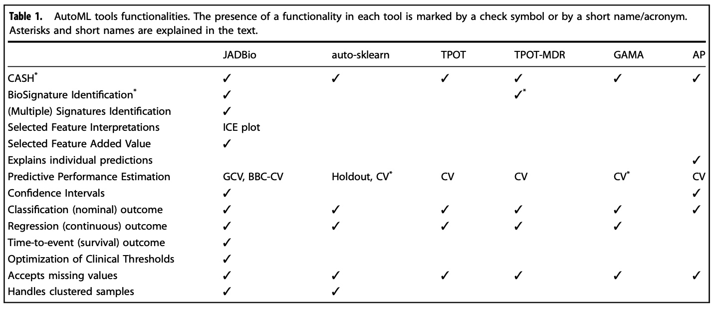
*See research paper for details on asterisks
Data and methodology used for the comparison
360 high-dimensional datasets, including transcriptomics (271 microarray, 23 RNA-seq), epigenomics (23), and metabolomics (43) data. The datasets are related to 125 diseases or phenotypes, with cellular proliferation diseases (i.e., different types of cancers) being the most represented group with 154 datasets. JADBio optimized for four different criteria, namely Performance (JADBio-P), Interpretability (JADBio-I), Feature Selection (JADBio- FS), and Aggressive Feature Selection (JADBio-AFS). We compare against auto-sklearn17, TPOT18, GAMA20, AutoPrognosis21, and Random Forest (RF22, scikit-learn implementation31). Each dataset was partitioned into two equal-size sample sets, each serving as the train and test set, respectively, leading to a total of 720 analyses. Further details in the Methods.
Results
Quantitative study: JADBio enables knowledge discovery and provides highly predictive models
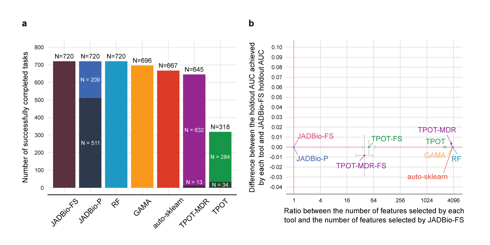
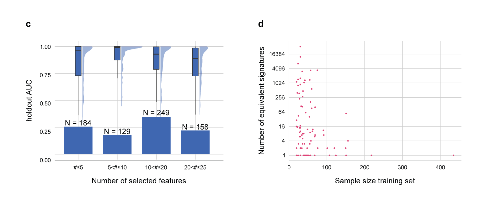
Fig. 4 Results of the quantitative comparison in terms of predictive performance.
a. Number of successfully completed tasks out of 720 for each tool. AutoPrognosis never completes any run and is not shown. JADBio-P and TPOT-MDR do attempt feature selection. The portion of runs where feature selection led to a winning model is depicted with a darker shade in their respective columns. JADBio-FS always enforces feature selection.
b. Comparison between JADBio-FS and all other tools in terms of relative dimensionality reduction and performance gain. The dimensionality reduction with respect to JADBio-FS (x-axis) is computed as the ratio between the number of features selected by each tool and the number of features selected by JADBio-FS (log2 scale). Values larger than one indicate that the tool selects more features than JADBio. The performance gain is reported on the y-axis, and it is computed as the difference between the holdout AUC achieved by each tool and the holdout AUC achieved by JADBio-FS. Values larger than zero indicate that the tool performs better than JADBio-FS. For each tool, we plot a point on the median values for each axis. Errors bars showing the standard error are shown. The median values are computed only on the completed runs. Cranberry-colored lines denote the baseline value, i.e., relative dimensionality reduction equal to one and performance gain equal to zero.
c. Holdout AUC distribution for JADBio-FS over different number of selected features. The holdout AUC distribution is reported both as a box and violin plot.
d. Contrasting the sample size in the training set (x-axis) and the number of equivalent signatures identified by JADBio-FS (y-axis, log2 transformed). Only runs where an algorithm able to identify multiple signatures was selected are shown. More than one signature was identified in a total of 68 runs out of 98, represented by the points with y coordinate larger than 1.
The results show that JADBio leads to models that require about 4000 fewer biomarkers to measure to achieve comparable predictive performance against all other tools included in the experiments.
Quantitative study: JADBio avoids overestimating performances
We investigate whether performance estimates obtained from the training set accurately reflect the ones computed on the holdout set. This is important to correctly assess the clinical usefulness of a model.
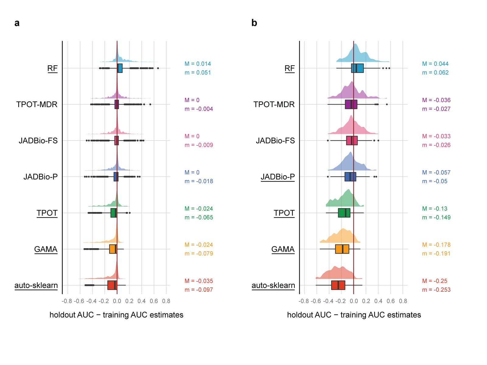
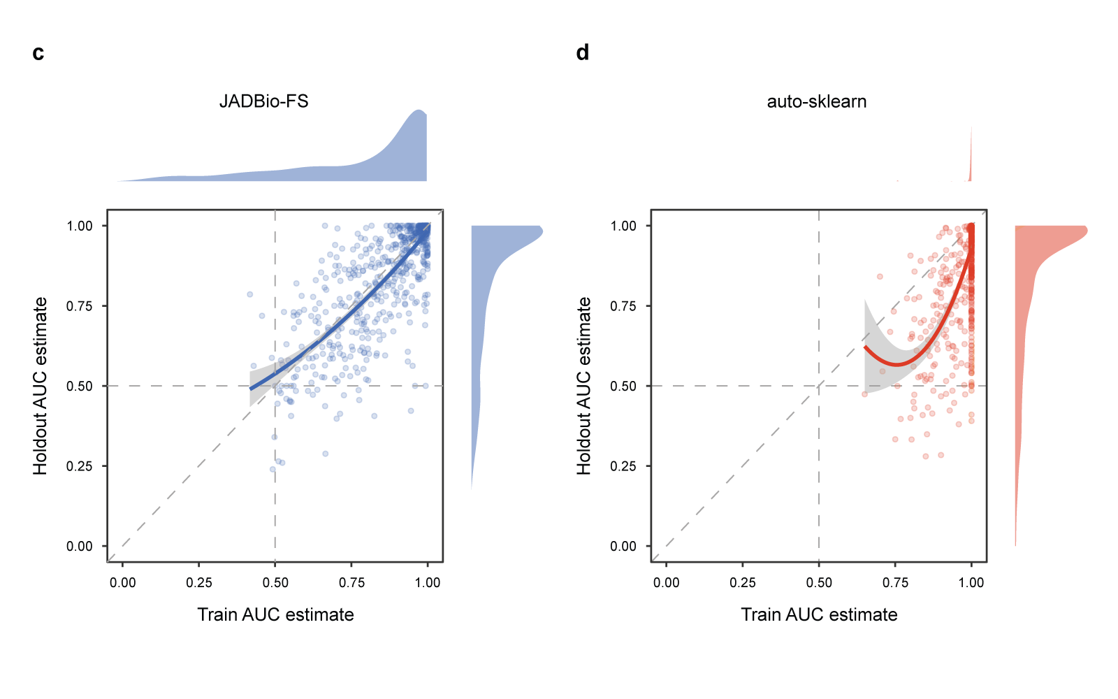
Fig 5 Results of the quantitative comparison in terms of bias.
Bias is defined as the holdout AUC estimate minus the AUC estimated on the training set; distributions on the right of the zero line correspond to conservative estimates, while results on the left of the line are optimistic. a. AUC bias distribution across 720 classification tasks (2 tasks for each of the 360 datasets). The distribution for each tool is reported both as a box and violin plot. Tools with median bias statistically significantly different from zero have their name underscored. Median (M) and average (m) bias values are reported on the right of each boxplot axis. b. Same as a, but only for the 196 runs where Random Forest (RF) achieves less than 0.8 AUC on the holdout set. On these more difficult tasks, TPOT, GAMA, and auto sklearn systematically overestimate performance between 14 and 25 AUC points. c. and d. Scatterplots reporting the AUC estimated on the training set (x-axis) vs. the AUC estimated on the holdout set (y-axis) for the JADBio-FS and auto-sklearn tools, respectively. Each point corresponds to one run. Locally Weighted Scatterplot Smoothing (LOESS) regression lines indicate the main trends in the corresponding scatterplot. Auto-sklearn points and LOESS line are mostly below the diagonal, indicating systematically overoptimistic performance estimates on the training set. The bias is significantly reduced for JADBio-FS, as indicated by a LOESS regression line close to the diagonal.
Panels (c) and (d) of Fig. 5 better visualize the difference in estimation properties between AutoML platforms. Each dot corresponds to a single run, where the x-axis reports the AUC estimate on the training set and the y-axis the estimate on the holdout set. The estimated training AUC is plotted against the achieved holdout AUC. Points above/below the diagonal corre- spond to runs underestimating/overestimating performance. The LOESS regression lines are shown in bold. Notice that auto-sklearn almost always overestimates performance. The stripe of dots on the right of the panel corresponds to auto sklearn estimates of exactly AUC = 1, while their holdout AUCs range from less than 0.5 to a perfect score of 1. In contrast, JADBio-FS runs are symmetrically distributed around the diagonal demonstrating that JADBio-FS estimates from the training set are on average accurate (zero bias). Of course, there is still variance in the estimation, which is why JADBio also reports confidence intervals. Other JADBio settings have more conservative performance estimates than JADBio-FS, possibly due to lower numbers of configurations explored (Supplementary Table 9).
In summary, these results indicate that JADBio provides reliable generalization performance estimates from the training set alone, while auto sklearn, GAMA, and TPOT fail in this respect.
CONCLUSIONS
- JADBio provides useful automation and functionality for translational research, predictive modeling, and corresponding decision support. Ana- lyses handled may involve multi-omics data complemented with clinical, epidemiological, and lifestyle factors resulting in hundreds of thousands of measured quantities. Low-sample size (<40) can be handled as well; while the variance in predictive performance can be large, the user can still gauge the clinical utility of the results by the reported confidence intervals. In general, no statistical knowledge or expertise is required, nor any computer programming abilities. However, some basic statistical knowledge is still necessary to fully interpret all reported metrics and graphs. Special emphasis is placed on facilitating biological interpretation and clinical translation.
- AutoML platforms automate the production of predictive models; they often lack other important functionality for translational research. The researchers argue that the current view of AutoML is to automate the delivery of a model, rather than to provide the full range of information required for successful interpretation and application of the model. In their opinion, this perspective is better described by the terms CASH (combined algorithm selection and hyperparameter optimization) or HPO (hyper-parameter optimization) and not AutoML. AutoML should instead be a term that implies automation at a different level, ideally delivering all information and insight that a human expert would deliver. JADBio is a step towards this direction, although of course, still far from fully realizing this vision.A major AutoML functionality of JADBio that is missing from other AutoML tools is feature selection (biosignature identification, biomarker discovery), i.e., identifying a minimal-size subsets of biomarkers that are jointly optimally predictive. Feature selection is often the primary goal of the analysis. The selected features lead to biological insights, cost-effect multiplex assays of clinical value, and identification of plausible drug targets. Feature selection is a notoriously difficult and combinatorial problem: markers that are not predictive in isolation (high unconditional p-value) may become predictive when considered in combination with other markers. The reverse also holds: markers that are predictive in isolation (low unconditional p-value), may become redundant given the selected features (high conditional p-value). JADBio embeds feature selection in the analysis process that scales to hundreds of thousands of features often encountered in (multi)-omics studies. GAMA and auto-sklearn do not attempt feature selection at all, while TPOT and TPOT-MDR do try feature selection methods, but they lead to the winning model only occasionally (11% and 2% of the times).Even more challenging is the problem of multiple feature selection, i.e., identifying all multiple feature subsets of minimal size that lead to optimally predictive models. In the case-study above, there were three feature subsets identified in the FR cohort (Fig. 3a), of five microbe species each, that lead to equally predictive models. Each one suffices for predictive purposes. But, when feature selection is used for knowledge discovery, it is misleading not to report all three signatures. In addition, identifying all of them provides design choices to the engineer of a diagnostic assay. The multiple feature selection problem has so far received relatively little attention by the community with only a handful of algorithms available. JADBio is the only tool offering this type of functionality.
- JADBio can significantly reduce the number of selected features (biomarkers) without compromising model quality in typical omics studies. This claim is supported by Fig. 4 and Supplementary Table 4, showing that when feature selection in JADBio is enforced (shown as JADBio-FS) the median AUC is decreased by only 0.0034 points with respect to the leading performing tool, namely TPOT-MDR, while the number of features selected is reduced by about ~4000 times. Interestingly, we note that Random Forests using the default settings can achieve predictive performance comparable with the results of much more sophisticated and computational-resource hungry CASH platforms on omics data. When predictive performance is the only goal in the analysis of an omics dataset, running solely Random Forests may suffice.
- JADBio provides accurate estimates of the out-of-sample performance with no need of an independent holdout set. This is supported by the results in Fig. 5 and Supplementary Table 6. The statement has the following serious ramifications: no samples need to be lost to estimating performance by the user. The final model is trained on all samples. JADBio automatically handles the estimation of perfor- mance and its uncertainty (confidence intervals). To clarify, we claim that the user does not need to hold out a separate test set to statistically validate the final model. This is of particular importance in omics datasets, often including a small number of patients due to rare conditions and cost. We would like to add the disclaimer however, that the estimates are valid only within the same operating environment. If batch effects or other distribu- tional changes are possible, a separate external validation set should be employed. This property of JADBio is necessary for full automation of analysis. Instead, the estimates by GAMA, TPOT, and auto-sklearn are shown to systematically overestimate (Fig. 5), arguably because such tools do not employ experimentation protocols devised for performance estimation on the training set.
What are the key ideas that enable JADBio to overcome key challenges?
The use of an AI decision-support system that encodes statistical knowledge about how to perform an analysis makes the system adaptable to a range of data sizes, data types, and user preferences. An automated search procedure in the space of appropriate combinations of algorithms and their hyper- parameter values, trying thousands of different machine learning pipelines (configurations) automatically optimizes choices. Proto- cols that estimate the out-of-sample predictive performance of each configuration, particularly the Generalized Cross Validation (see Methods) suitable for small sample sizes reduces the uncertainty (variance) of estimation. Treating all steps of the analysis (i.e., preprocessing→ imputation→ feature selection → predictive modeling) as an atom, and cross-validating configura- tions rather than just the final modeling step avoids over- estimation. A statistical method for removing the performance optimism (bias) due to trying numerous configurations (BBC-CV) is also necessary to avoid overestimation. The use of a feature selection algorithm that scales up to hundreds of thousands of biomarkers, suitable for small sample sizes allows the identifica- tion of multiple statistically equivalent biosignatures (SES algorithm).
As noted at the start, JADBio’s AutoML approach can accelerate precision medicine and translational research. Specifically, it could facilitate the discovery of novel biosignatures and biomarkers leading to new biological insights, precision medicine predictive models, drug targets, and non-invasive diagnostics in cancer or other conditions.
Read the full paper on npj | precision oncology: Just Add Data: automated predictive modeling for knowledge discovery and feature selection
OTHER
Do you have questions?
JADBio can meet your needs. Ask one of our experts for an interactive demo.
Stay connected to get our news first!
Do you have questions?
JADBio can meet your needs. Ask one of our experts for an interactive demo.

Join the JADai Community!
Sign up with a FREE Basic plan! Be part of a growing community of AutoML enthusiasts
GET STARTED


